Data From Fig 7d – LSD1 inhibition circumvents glucocorticoid-induced muscle wasting of male mice
Two interesting bits with Fig 7d: 1) The researchers analyzed figure 7b data using one-way ANOVA with Tukey adjustment. Post-hoc p-value adjustment is common but typically unjustified for bench biology data like these. The example is a good one to talk about p-value adjustment in bench biology. 2) The linear/ANOVA model implies absurd inference from the CI/SE error bars, including mean counts less than zero!
p-values
multiple testing
generalized linear model
absurd CI
power
simulation
pseudoreplication
analysis flag
Author
Jeff Walker
Published
June 25, 2024
Modified
October 2, 2024
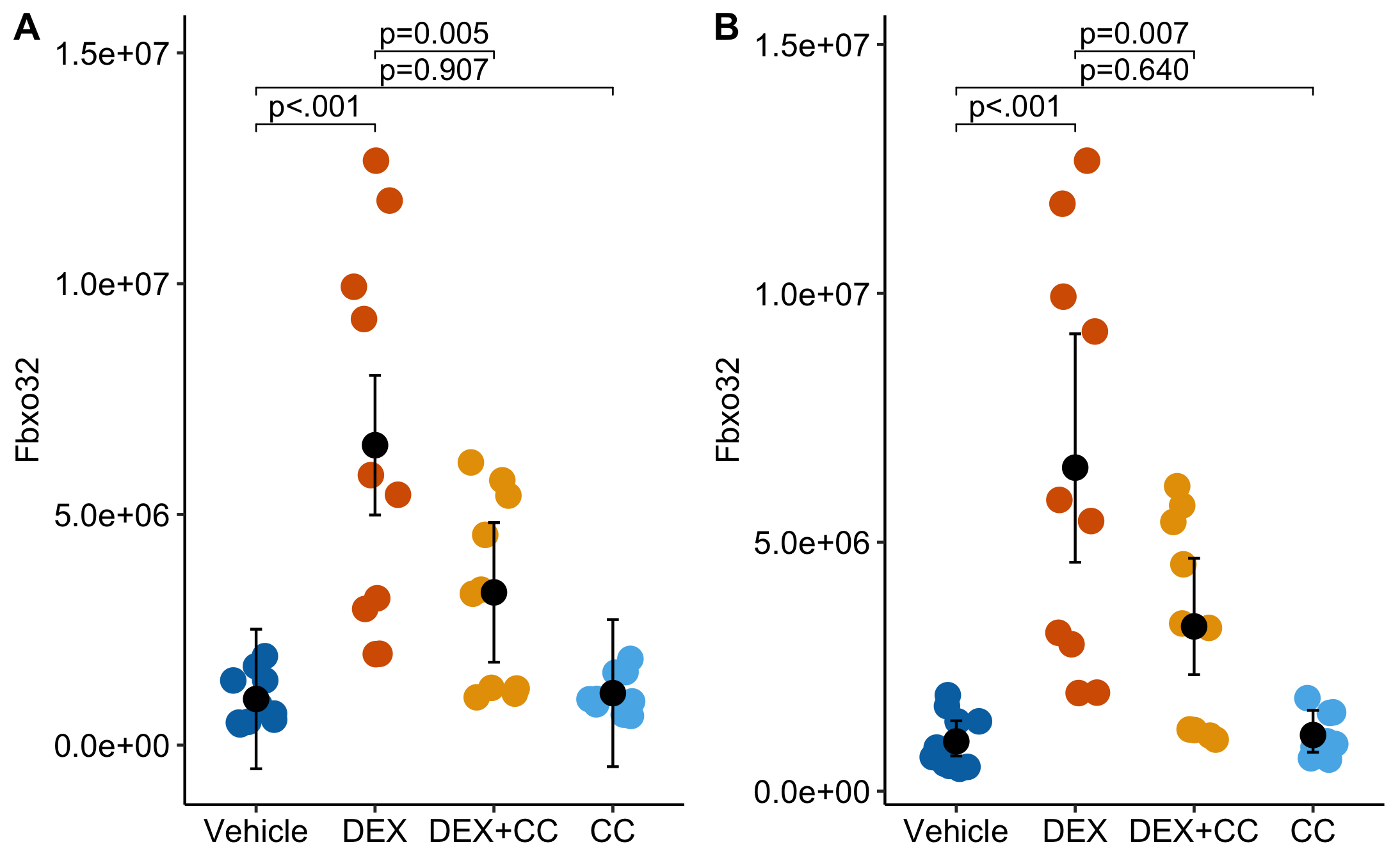
(A) Reproduced published plot using ANOVA model. Note the modeled CIs imply negative counts and absurd variances. (B) Better-than-reproduced plot using NB-GLM modeled CIs that don’t dip below zero and reflect true variance among groups.
Dexamethasone (DEX) is a synthetic glucocortacoid hormone used to treat inflammation and chronic autoimmune diseases but it also stimulates muscle atrophy. The authors are investigating the role of interactions between Lysine-specific demethylase 1 (LSD1) and the glucocortacoid recepter (GCR) in the development of muscle atrophy.
Earlier experiments presented in the paper show evidence that atrophy is mediated by a LSD1/GCR complex that regulates genes related to atrophy and other pathways. For this experiment, mice were treated with a combination of DEX and the LSD1-specific inhibitor CC-90011. Here the researchers are looking at the effect of the different treatment combinations on RNA expression of genes related to the ubiquitin-proteasome system (Fbxo32, Trim63) and the autophagy system (Atg7, Becn1, Bnip3).
Treatment levels
Vehicle (Dex-/CC-) Expected to have low levels of target gene expression
Dex (Dex+/CC-) Positive control. Expected to have elevated levels of target gene expression relative to vehicle
CC (Dex-/CC+) Important negative control. We expect this to be similar to Vehicle. If it is not, we need the interaction.
DEX+CC (Dex+/CC+) If LSD1 works with the GCR as expected, then we expect these levels to be lower than Dex+/CC- but how much depends on CC concentration.
Analysis Flag: The data are two technical replicates per mouse, so all inference will be a little optimistic. The mouse ID was not archived so I cannot better-than-reproduce the results.
Setup
Import and Wrangle
Code
data_from <-"LSD1 inhibition circumvents glucocorticoid-induced muscle wasting of male mice"file_name <-"41467_2024_47846_MOESM4_ESM.xlsx"file_path <-here(data_folder, data_from, file_name)read7d <-function(range_val ="B3:E13", label_val ="Fbxo32"){ fig7d_part <-read_excel(file_path,sheet ="Fig. 7d",range = range_val,col_names =TRUE) |>data.table() |>melt(variable.name ="excel_label", value.name ="y")# un-normalize count by multiplying by 10^6 fig7d_part[, y :=as.integer(y *10^6)]setnames(fig7d_part, old ="y", new = label_val) fig7d_part[, mouse_id :=paste0("mouse_", .I)]return(fig7d_part)}fig7d <-read7d(range_val ="B3:E13", label_val ="Fbxo32")fig7d <-merge(fig7d,read7d(range_val ="B16:E26", label_val ="Trim63"),by =c("excel_label", "mouse_id"))fig7d <-merge(fig7d,read7d(range_val ="B29:E39", label_val ="Atg7"),by =c("excel_label", "mouse_id"))fig7d <-merge(fig7d,read7d(range_val ="B42:E52", label_val ="Becn1"),by =c("excel_label", "mouse_id"))fig7d <-merge(fig7d,read7d(range_val ="B55:E65", label_val ="Bnip3"),by =c("excel_label", "mouse_id"))# remove the missing countfig7d <-na.omit(fig7d)# better treatment labels than in excel filefig7d[excel_label =="Ctrl Oil", treatment :="Vehicle"]fig7d[excel_label =="DEX", treatment :="DEX"]fig7d[excel_label =="DEX+CC-90011", treatment :="DEX+CC"]fig7d[excel_label =="CC-90011", treatment :="CC"]fig7d[, treatment :=factor(treatment, levels =unique(fig7d$treatment))]# split treatment into two factorsfig7d[treatment =="Vehicle", dex :="Dex_neg"]fig7d[treatment =="Vehicle", cc :="CC_neg"]fig7d[treatment =="DEX", dex :="Dex_pos"]fig7d[treatment =="DEX", cc :="CC_neg"]fig7d[treatment =="DEX+CC", dex :="Dex_pos"]fig7d[treatment =="DEX+CC", cc :="CC_pos"]fig7d[treatment =="CC", dex :="Dex_neg"]fig7d[treatment =="CC", cc :="CC_pos"]fig7d[, dex :=factor(dex, levels =c("Dex_neg", "Dex_pos"))]fig7d[, cc :=factor(cc, levels =c("CC_neg", "CC_pos"))]file_out_name <-"LSD1 inhibition circumvents glucocorticoid-induced muscle wasting of male mice.xlsx"fileout_path <-here(data_folder, data_from, file_out_name)write_xlsx(fig7d, fileout_path)
Does the unstandardization matter
Code
Fbxo32_4 <- fig7d[, Fbxo32]/10^6*10^4m1 <-lm(Fbxo32 ~ treatment, data = fig7d)m2 <-lm(Fbxo32_4 ~ treatment, data = fig7d)coef(summary(m1))
The reported p-values are conservative (a bit on the “multiple testing” problem), or not!
The researchers reported Tukey-adjusted p-values. The Tukey method adjusts for the number of tests in a “family” of tests, where a family is the set of tests that answer one question. The researchers follow the norm in bench bio and choose the whole set of six contrasts as the family. This would answer a question such as: “if we were to create these combinations, would we find any difference between at least on pair?”, which isn’t a very interesting question.
The researchers are focused on a much more specific question and at least two more questions, both related to controls:
Family 1: Is there evidence that CC attenuates DEX-induced expression? There is only one test in this family: DEX+CC - DEXI. This is the focal family.
Family 2: Is there evidence that DEX increase expression levels, as expected? This is the “positive control” family. There is only one test in this family: DEX - Vehicle.
Family 3: What is the effect of CC alone? This is “negative control” family. Without DEX-induced elevated express, we would expect this response to be similar to Vehicle. There is only one test in this family: CC - Vehicle.
What about the interaction effect? The contrast (DEX+CC - DEX) is the focal contrast if there is no effect of CC alone. We could look at the CC alone effect (CC - Vehicle) and if it is sufficiently small, use (DEX+CC - DEX) as the focal contrast. Of course “sufficiently small” has a subjective bright line. The statistically correct way to address this is to compare the effect of CC with DEX (the focal contrast) to the effect of CC without DEX (CC - Vehicle). This comparison is the interaction effect. So we’ll add the interaction contrast as a 4th family, which we should think of as replacing the focal contrast (Family 1) and not “in addition to” the three families. But, I’ll compute both. Regardless, for these data, I think most researchers would agree that CC - Vehicle is sufficiently small that we can use the DEX+CC - DEX comparison without issue.
So we have three p-values that we care about and each is from a different family, so there is no justification for p-value adjustment for multiple tests. This would make the reported p-values conservative. In general, if I wanted to be more conservative, in order to avoid research time and waste, I’d simply make my “alpha” smaller, such as 0.01 or 0.005 instead of using more conservative tests like a Tukey p-value adjustment, since the conservative alpha doesn’t depend on things like number of tests in a family.
Code
# the researcher's analysism0 <-lm(Fbxo32 ~ treatment, data = fig7d)m0_emm <-emmeans(m0, c("treatment"))m0_pairs <-contrast(m0_emm,method ="revpairwise",adjust ="tukey") |>summary(infer =TRUE)# the analysis only comparing the families of tests that we care aboutveh =c(1, 0, 0, 0)dex =c(0, 1, 0, 0)dex_cc =c(0, 0, 1, 0) # note the wonky ordering in fig 7dcc =c(0,0,0,1)focal_contrasts =list("DEX - Vehicle"= dex - veh,"CC - Vehicle"= cc - veh,"DEX+CC - DEX"= dex_cc - dex,"interaction"= (dex_cc - dex) - (cc - veh))m1 <-lm(Fbxo32 ~ treatment, data = fig7d)m1_emm <-emmeans(m1, c("treatment"))m1_pairs <-contrast(m1_emm,method = focal_contrasts,adjust ="none") |>summary(infer =TRUE)contrast_table <-rbind(m0_pairs, m1_pairs)contrast_table |>kable(digits =4) |>kable_styling() |>pack_rows("Adjusted", 1, 6) |>pack_rows("Non-adjusted", 7, 10)
contrast
estimate
SE
df
lower.CL
upper.CL
t.ratio
p.value
Adjusted
DEX - Vehicle
5499807.1
1053488
35
2658652.5
8340961.7
5.2206
0.0000
(DEX+CC) - Vehicle
2310044.2
1053488
35
-531110.4
5151198.8
2.1928
0.1452
(DEX+CC) - DEX
-3189762.9
1053488
35
-6030917.5
-348608.3
-3.0278
0.0228
CC - Vehicle
127648.4
1082356
35
-2791360.5
3046657.2
0.1179
0.9994
CC - DEX
-5372158.7
1082356
35
-8291167.6
-2453149.9
-4.9634
0.0001
CC - (DEX+CC)
-2182395.8
1082356
35
-5101404.7
736613.0
-2.0163
0.2015
Non-adjusted
DEX - Vehicle
5499807.1
1053488
35
3361112.9
7638501.3
5.2206
0.0000
CC - Vehicle
127648.4
1082356
35
-2069651.1
2324947.8
0.1179
0.9068
DEX+CC - DEX
-3189762.9
1053488
35
-5328457.1
-1051068.7
-3.0278
0.0046
interaction
-3317411.3
1510408
35
-6383701.9
-251120.7
-2.1964
0.0348
The top table contains the six Tukey-adjusted p-values reported by the researchers. The bottom table contains the unadjusted values of only the contrasts of interest. The adjusted p-value for the focal contrast DEX+CC - DEX is 0.023 while the unadjusted value is 0.0046.
The p-value of the interaction is 0.035 – note that it’s effect size is very similar to that of the DEX+CC - DEX but the p-value is bigger because the SE of an interaction is bigger than the SE of a main contrast (because the interaction is a function of 4 means and not just 2). Using the interaction p-value is not just statistically correct, it is more conservative.
Fig7d is a good example of how a linear/ANOVA model for count data often implies silly confidence intervals
The two plots above are the estimated means and 95% CIs from the linear/ANOVA model (A) and a negative-binomial Generalized Linear Model (B). The linear/ANOVA model implies two absurd things about the confidence of the means of the groups
Homogeneity of variances – remember, equal variance among treatment levels is an assumption of a linear/ANOVA model, so the model standard error of the mean of a group is a function only of the group sample size. The modeled SEs/CIs are too big for the groups with small mean counts and too small for the groups with large mean counts.
Values below zero. A good way to think about a CI is, values within a confidence interval are reasonably plausible values for the group mean. The CIs of Vehicle and CC imply that negative means are “reasonably plausible” values, which is absurd, counts cannot be negative.
By contrast, the CIs from the GLM more accurately model the data.
The modeled CIs vary among the groups and look much more like the sampled CIs. In a negative-binomial GLM, the model standard error of the mean of a group is a function of the sample size and the mean of the group – groups with larger means have larger variances/standard errors. It’s easy to see this phenomenon with these data; the spread of points for DEX is much more than that for Vehicle, but the linear/ANOVA model CIs do not model this.
the CIs are asymmetric, the upper bound is further from the mean than the lower bound. Again, this reflects the skew of the data.
the CIs do not (and cannot) dip below zero.
We don’t see figures like Panel A above because researchers plot sample SEs and not modeled SEs – the SE actually used to compute the p-value. So “inference from the plot” is inconsistent with the p-value. This is why researchers should plot the model (modeled SE/CI) and not the data (sampled SE/CI).
A bit more about Generalized Linear Models (GLM)
Count data in biology often have a distribution that nicely approximates a sample from a Negative Binomial or a Quasipoisson distribution. Two features of count data that violate assumptions of a linear/ANOVA model are
Homeogeneity of variance – the variance of the response is proportional to the mean of the group, so groups with a higher mean count have higher variances
Normal – counts are right skewed, that is, there is a high density of low counts and a low density of high counts
Generalized Linear Models (GLM) were developed to compute confidence intervals and p-values for counts and other kinds of data with non-normal distributions.
For these data, the Linear/ANOVA model has more power than a Negative-Binomial GLM
Despite the violations, tests from linear/ANOVA models that give a p-value often have good long-run performance, that is, they have relatively high power and controlled type I error Ives 2015. GLM models for count data can have higher power than a linear/ANOVA model, but this sometimes requires some more sophisticated methods such as bootstrap resampling Warton et al. 2016.
Here I use a simulation to compare the Type I error and Power of the 1) Linear/ANOVA model, 2) a Negative Binomial GLM, and 3) a quasipoisson GLM for data that look like those in Figure 7d. I explicitly simulate the Trim63 response with the same unbalanced data as in the experiment (the CC group only has 9 measures and not 10).
Code
# get parametersdo_it <-FALSEif(do_it){ data_params <- fig7d[, .(mean =mean(Trim63),N = .N), by ="treatment"] mu <-rep(data_params$mean, data_params$N) N <-sum(data_params$N) m1 <-glm.nb(Trim63 ~ dex * cc, data = fig7d) theta_sim <- m1$theta n_sim <-2000 fd <-data.table(treatment =rep(c("veh", "dex", "dex_cc", "cc"), data_params$N),dex =rep(c("no_dex", "dex", "dex", "no_dex"), data_params$N),cc =rep(c("no_cc", "no_cc", "cc", "cc"), data_params$N),Trim63 =as.numeric(NA) )# power power_matrix <-matrix(nrow = n_sim, ncol =6)colnames(power_matrix) <-c("lm_focal", "lm_ixn", "nb_focal", "nb_ixn", "qp_focal", "qp_ixn")for(sim_i in1:n_sim){# fake data fd[, Trim63 :=rnegbin(N, mu, theta_sim)]# lm/ANOVA m_lm <-lm(Trim63 ~ dex * cc, data = fd) power_matrix[sim_i, "lm_ixn"] <-coef(summary(m_lm))["dexno_dex:ccno_cc", "Pr(>|t|)"] m_lm_pairs <-emmeans(m_lm, specs =c("dex", "cc")) |>contrast(method ="revpairwise", simple ="each", combine =TRUE, adjust ="none") |>summary(infer =TRUE) power_matrix[sim_i, "lm_focal"] <- m_lm_pairs[3, "p.value"] # effect of CC when dex is present# glm neg bin m_nb <-glm.nb(Trim63 ~ dex * cc, data = fd) power_matrix[sim_i, "nb_ixn"] <-coef(summary(m_nb))["dexno_dex:ccno_cc", "Pr(>|z|)"] m_nb_pairs <-emmeans(m_nb, specs =c("dex", "cc")) |>contrast(method ="revpairwise", simple ="each", combine =TRUE, adjust ="none") |>summary(infer =TRUE) power_matrix[sim_i, "nb_focal"] <- m_nb_pairs[3, "p.value"] # effect of CC when dex is present# glm quasipoisson m_qp <-glm(Trim63 ~ dex * cc,family =quasipoisson(link ="log"),data = fd) power_matrix[sim_i, "qp_ixn"] <-coef(summary(m_qp))["dexno_dex:ccno_cc", "Pr(>|t|)"] m_qp_pairs <-emmeans(m_qp, specs =c("dex", "cc")) |>contrast(method ="revpairwise", simple ="each", combine =TRUE, adjust ="none") |>summary(infer =TRUE) power_matrix[sim_i, "qp_focal"] <- m_qp_pairs[3, "p.value"] # effect of CC when dex is present }# type I type1_matrix <-matrix(nrow = n_sim, ncol =6)colnames(type1_matrix) <-c("lm_focal", "lm_ixn", "nb_focal", "nb_ixn", "qp_focal", "qp_ixn")for(sim_i in1:n_sim){# fake data fd[, Trim63 :=rnegbin(N, mu[1], theta_sim)]# lm/ANOVA m_lm <-lm(Trim63 ~ dex * cc, data = fd) type1_matrix[sim_i, "lm_ixn"] <-coef(summary(m_lm))["dexno_dex:ccno_cc", "Pr(>|t|)"] m_lm_pairs <-emmeans(m_lm, specs =c("dex", "cc")) |>contrast(method ="revpairwise", simple ="each", combine =TRUE, adjust ="none") |>summary(infer =TRUE) type1_matrix[sim_i, "lm_focal"] <- m_lm_pairs[3, "p.value"] # effect of CC when dex is present# glm neg bin m_nb <-glm.nb(Trim63 ~ dex * cc, data = fd) type1_matrix[sim_i, "nb_ixn"] <-coef(summary(m_nb))["dexno_dex:ccno_cc", "Pr(>|z|)"] m_nb_pairs <-emmeans(m_nb, specs =c("dex", "cc")) |>contrast(method ="revpairwise", simple ="each", combine =TRUE, adjust ="none") |>summary(infer =TRUE) type1_matrix[sim_i, "nb_focal"] <- m_nb_pairs[3, "p.value"] # effect of CC when dex is present# glm quasipoisson m_qp <-glm(Trim63 ~ dex * cc,family =quasipoisson(link ="log"),data = fd) type1_matrix[sim_i, "qp_ixn"] <-coef(summary(m_qp))["dexno_dex:ccno_cc", "Pr(>|t|)"] m_qp_pairs <-emmeans(m_qp, specs =c("dex", "cc")) |>contrast(method ="revpairwise", simple ="each", combine =TRUE, adjust ="none") |>summary(infer =TRUE) type1_matrix[sim_i, "qp_focal"] <- m_qp_pairs[3, "p.value"] # effect of CC when dex is present }saveRDS(power_matrix, "power_matrix.Rds")saveRDS(type1_matrix, "type1_matrix.Rds")}else{ power_matrix <-readRDS("power_matrix.Rds") type1_matrix <-readRDS("type1_matrix.Rds")}pless <-function(x){ stat <-sum(x <0.05)/length(x)return(stat)}res <-data.table(Test =c("LM: DEX+CC - DEX", "LM: Interaction","GLM-NB: DEX+CC - DEX", "GLM-NB: Interaction","GLM-QP: DEX+CC - DEX", "GLM-QP: Interaction"),Power =apply(power_matrix, 2, pless),"Type I"=apply(type1_matrix, 2, pless))res |>kable() |>kable_styling(full_width =FALSE)
Test
Power
Type I
LM: DEX+CC - DEX
0.8120
0.0520
LM: Interaction
0.6930
0.0475
GLM-NB: DEX+CC - DEX
0.7340
0.0745
GLM-NB: Interaction
0.6970
0.0685
GLM-QP: DEX+CC - DEX
0.7935
0.0575
GLM-QP: Interaction
0.5595
0.0490
Curious. The linear model with an untransformed response has better Type I control and slightly more power than a negative binomial GLM.
That said, I really like the GLM for two reasons:
The effect is a multiple of the reference, which is a really meaningful way of comparing responses (for example, looking at the table below, the effect is 6.5, meaning the expression level is 6.5 times larger than that of Vehicle)
The CIs of the means are asymmetric, which reflects the skewed distribution of the data. This also avoids absurd CIs such as a negative lower bound (counts can’t be negative!).